Dive In - Make a Graph

Video Demonstration of Making a Graph¶

Get Started¶

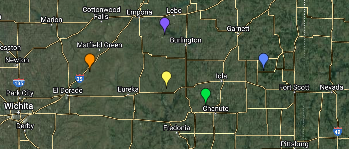
To make a time series graph with Climate Engine, first you need to select the “Make Graph” tab. This tab shows an interactive panel. Immediately, you will get a point marker on the map. You can use this to select your location/region of interest.

Selecting a Time Series Calculation¶

First, you need to select the type of plot. Climate Engine allows you to generate and customize three kinds of time series figures.

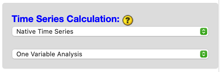
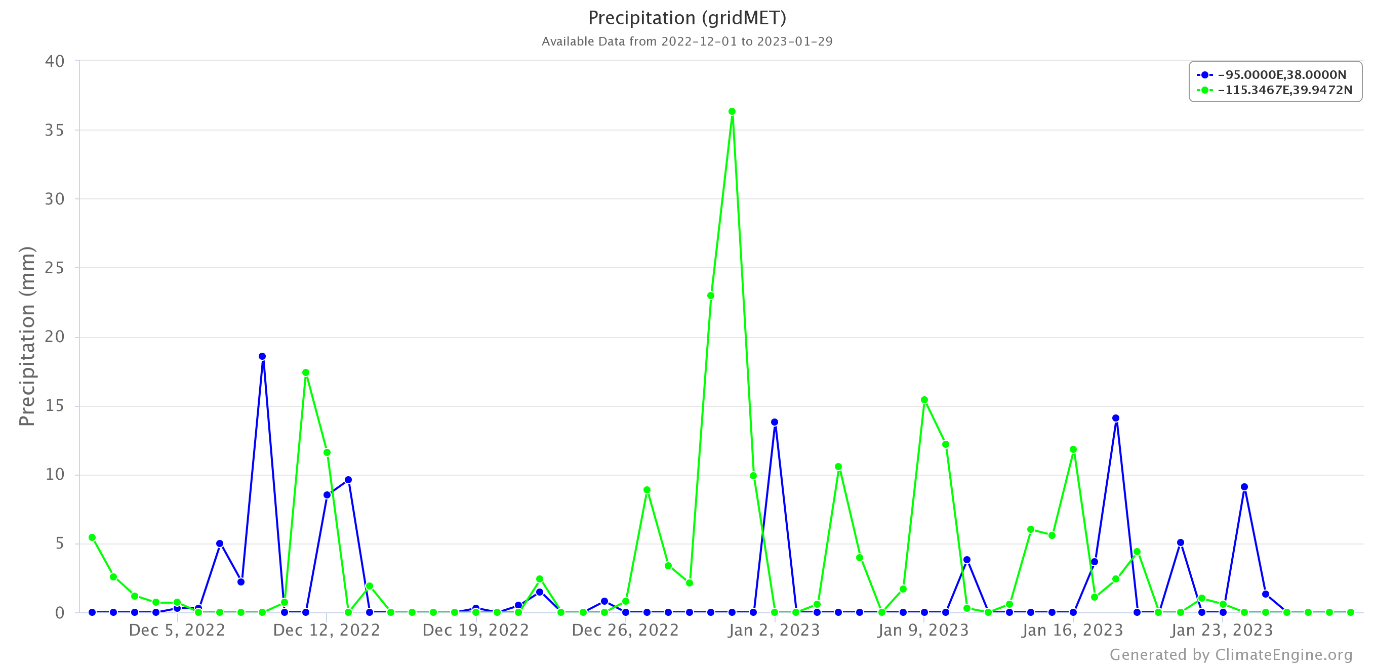
Native Time Series: Plots raw data over a specified time period at the native frequency of the selected dataset.

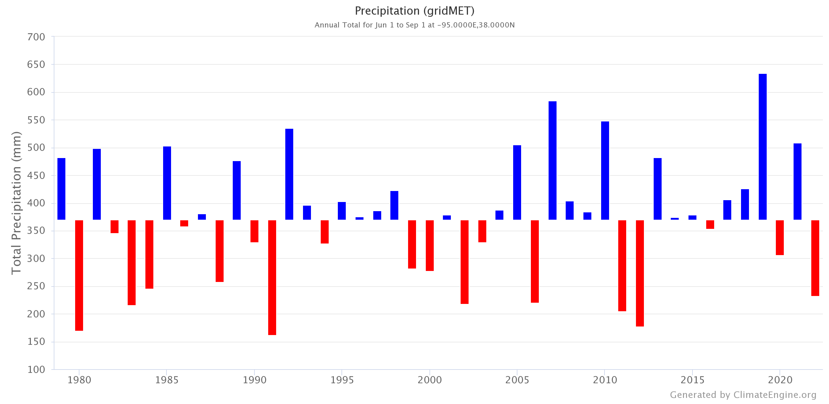
Summary Time Series: Plots yearly values computed over a uniform period within each year, as specified by the user, such as Winter or Annual averages.

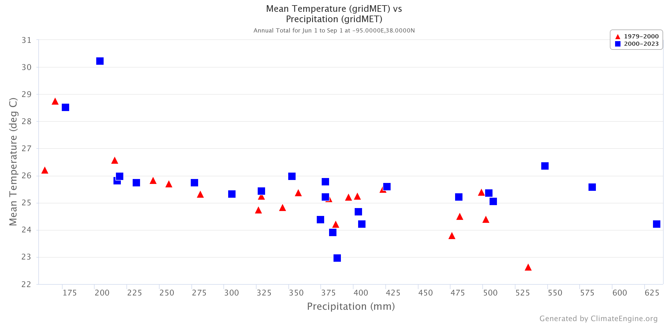
Two Variable Scatterplot: Plots two variables against each other over a uniform period within each year, as specified by the user, with the option to compare two time periods separately.

Climate Engine allows you to plot time series for either one variable (on the left y-axis) or two variables (one on the left y-axis and the other on the right y-axis). You need to select how many variables you would like to display at once, with caution that choosing two variables can lead to the plot sometimes getting messy.

Selecting Region(s) of Interest¶

Second, you have the option to select your region. The same kinds of time series can be produced by either a point location or an area average over a region.

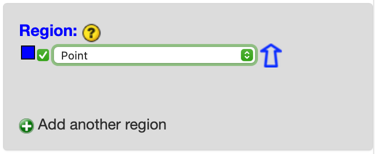
To choose a point location, first select Region > Point. Then drag and drop the marker at the point of interest. You can add up to four additional locations when doing the Native Time Series Calculation. To add another point, click the + icon next to “Add another region” to add another point. Drag and drop the new point to your location of interest. To remove a point location, you can 1) uncheck the checkbox next to the point you want to remove so it is not used in the time series, 2) double click on the point marker on the map to remove and uncheck it, and 3) click the - button to the right of the point to remove the entry.

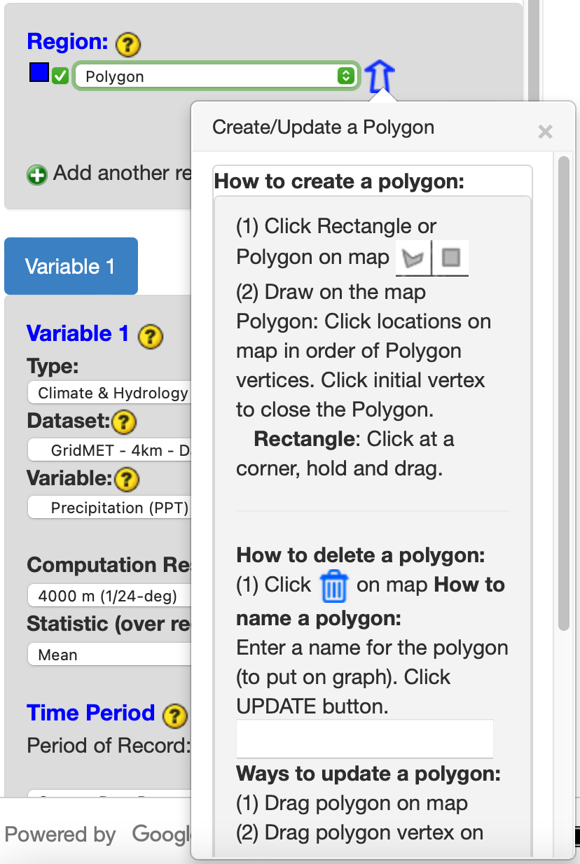
To analyze custom polygon regions, you have three options. The first, select Region > Polygon, allows you to draw the polygon or rectangle of interest. By clicking the blue arrow outline to the right, it allows you to enter a name for the polygon and adjust its coordinates. If you need to delete a polygon, you can click the blue trash can at the top center of the map. Similarly to points, you can add up to four additional polygons.

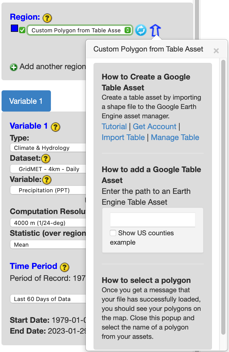
The second, select Region > Custom Polygon from Table asset, allows you to input an earth engine asset id. If the asset loads successfully, a success message will appear. Similarly, if the asset fails to load, a failure message will appear. It will then prompt you to select the Column Name to Import. Then a dropdown will appear that allows you to select individual polygons if the shapefile has multiple. Similarly to points and polygons, you can add up to four additional earth engine assets. See this article to learn more about creating a custom polygons from table assets.

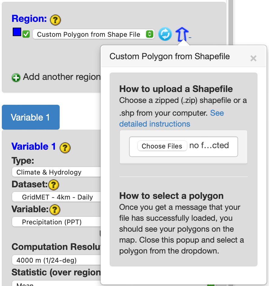
The third, select Region > Custom Polygon from Shapefile, allows you to upload a shapefile. It allows you to upload a zipped shapefile folder or .shp file from your computer. Once your shapefile is successfully uploaded, you will be prompted to select a column name to import. Then you will be able to select specific polygons via a dropdown. The polygon(s) selected will show up on the map outlined in black. 

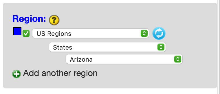
Lastly, the research app provides a variety of pre-loaded region choices to choose from. These include World Regions, US states, BLM Grazing Allotments, US Tribal Layers, etc. Once you select one of the preset choices, it populates dropdowns that allow you to select an individual region. The polygon(s) selected will show up on the map outlined in black. Another option to choose an individual region is by clicking on one of the states. Similarly to points and polygons, you can add up to four additional earth engine assets. To reset your selections, just click the light blue refresh button. 

Selecting Variables for Analysis¶

If you selected one variable analysis from the Time Series Calculation section, you will have a tab with “Variable 1” in it. If you chose two variable analysis, you will have two tabs with “Variable 1” and Variable 2” that you can toggle between.

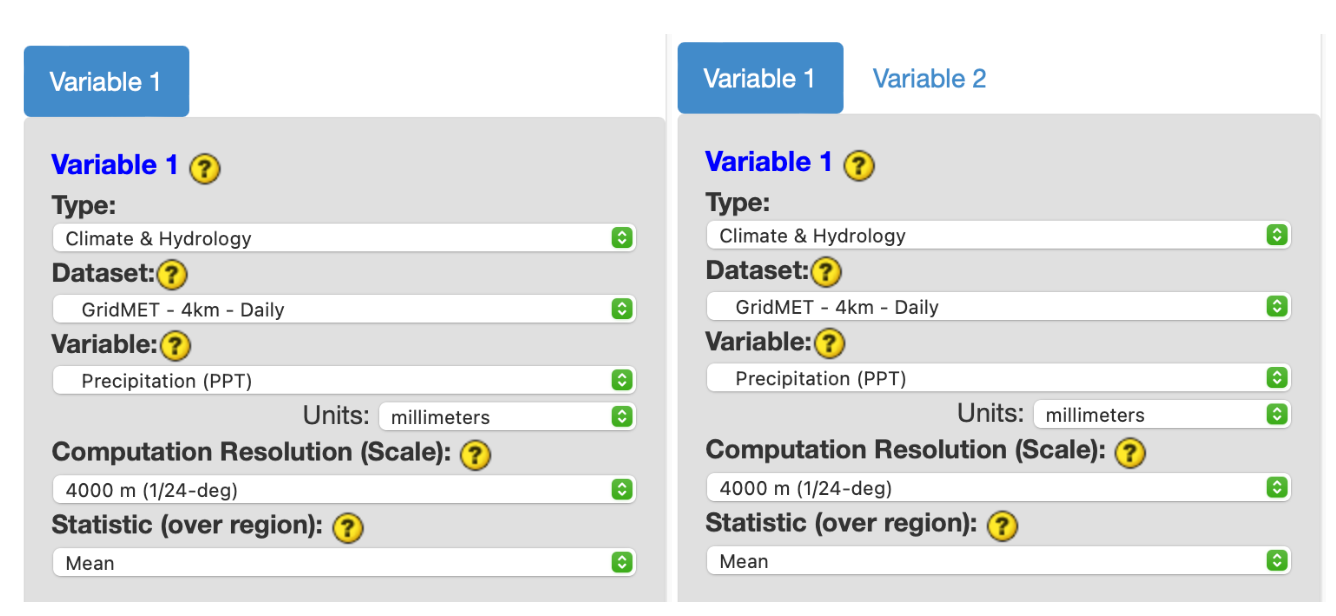
For each variable tab, you must first select the product type from amongst: “Climate & Hydrology”, “Remote Sensing”, “Hazards”,  and “Forecasts”. Once the product type is selected, the different datasets available within the product type will be populated in the “Dataset” dropdown. Clicking the yellow question mark next to the dataset will open a window with more information about that dataset. Once the dataset is selected, the different variable metrics available under the dataset will be populated in the “Variable” dropdown. The tabs also provide additional options for specifying computation resolution (scale) and statistic (over region). For time series, only raw values of the data plotted. So there is no option for plotting anomalies. For the scatterplots, variable 1 is placed on the x-axis and variable 2 is placed on the y-axis.

Optional Masking¶

This section allows two options: 1) No mask (shows all values on the map) and 2) Mask data by category (computes values within defined areas). If you used masking in the Make Map tab, this section may be already filled out. Selecting masks works the same for the Make Graph tab as the Make Map tab described above. The timeseries values will only reflect the desired areas according to the masking within the region, rather than values for the entire region. One important note is the timeseries masking only works for polygon regions. If you select a point, an error will be returned.

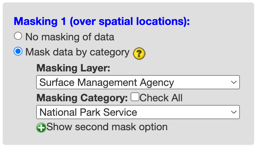
When you select the Mask data by category option, you are provided two drop-down menus. The first drop-down, Masking Layer, lists the masking layers you can select from. Once a masking layer is selected, the Masking Category drop-down will be populated with the categories to select from. Multiple categories can be selected and the resulting mask will be a union of those categories. If you are interested in all available categories you can click the Check All box. Then you can fill out the rest of the graphing panel as usual, including defining your “Region” and click Compute Time Series. The graph will display in the graph tab. Information about the mask is added to the figure caption.

Selecting Time Period for Analysis¶

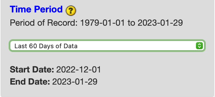
Climate Engine allows you to specify the time period you want to use for the time series. In this section of the data request tab, you will select a date range from the dataset to perform the above processing upon. The period of record is available above the date selection dropdown. 

The first option you have is to select a general time period you would like to look at, such as the last 60 days or the northern water year. In these cases, the date range will be automatically populated for you.

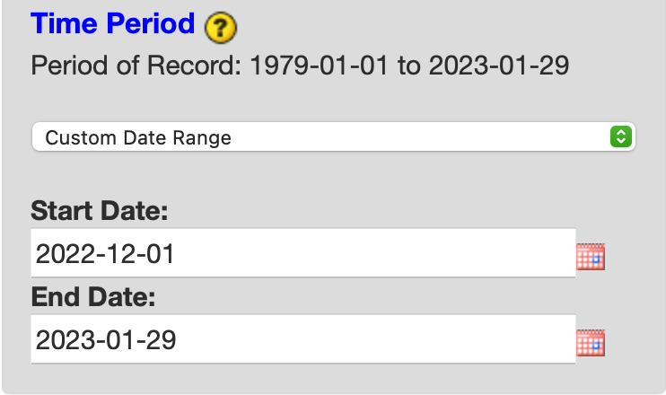
Second, if you would like to manually enter or adjust your date range, first select custom and then manually enter your date range via the text boxes or the calendar function.

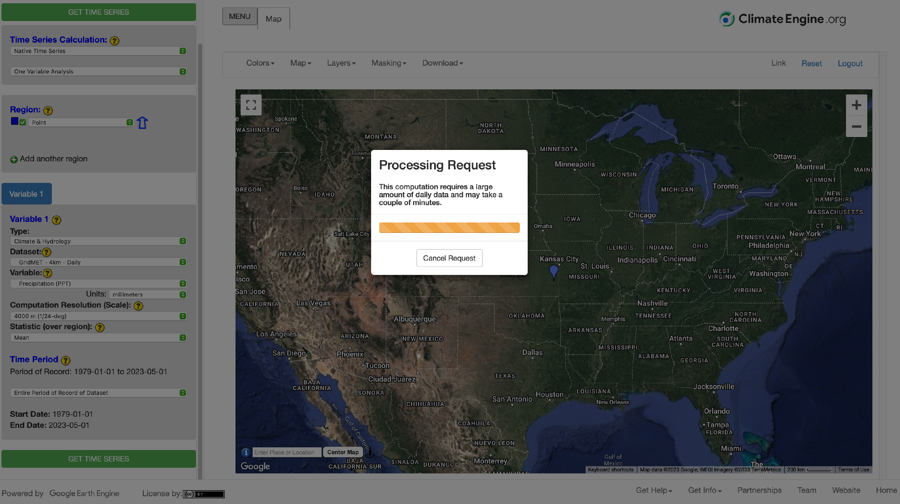
Submitting the Request¶

Once you have selected the time series calculation, the region(s) for your time series and the variable information (product, processing and time period), you are ready to create a time series.  To submit your request, click the green button ‘GET TIME SERIES’. Once you do this, a window will popup letting you know that the site is working to get your time series. For some requests, the time series figure will show up quickly. For other requests (i.e. those that require the download or processing of a lot of data), it may take a while.