Python Scripts

Scaling up your analysis with the Climate Engine API¶

Making API calls from python scripts allows you to integrate the the power of cloud computing with your existing workflows and automate iterative processes. Unlike the app, you can export time series for numerous areas of interest with a few lines of code.

Getting Set Up¶

First, at the top of your script you will want to import any packages you will need for making maps, charts, etc. The Climate Engine API itself doesn't require any packages to utilize. You will need two things to get set up to make API requests: 1) a root URL and 2) authorization key. Additionally, you can set your google bucket variable in this section.

# Import/Install Packages
import datetime
import os
import requests
import time

!pip install --quiet geopandas
import pandas as pd
import geopandas as gpd

import numpy as np
import matplotlib
import matplotlib.pyplot as plt

# Import/Install Packages
%%capture
if 'google.colab' in str(get_ipython()):
    !pip install --quiet rioxarray

#Install mapping packages
import rioxarray as rxr
from rioxarray.merge import merge_arrays
import matplotlib.pyplot as plt
from mpl_toolkits.axes_grid1 import make_axes_locatable

#Prep for API Call
# Set root URL for API requests
root_url = 'https://api.climateengine.org/'
# Authentication info for the API (do not share this widely)
headers = {'Authorization': 'Add Your API Key'}
# Google Storage bucket for storing output files
bucket_name = 'Add Your Bucket Name'

Requesting Rasters¶

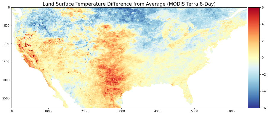
To request a raster, first you need to select the appropriate endpoint for you goals. To see all of the endpoint options, you can visit the Endpoint Parameters section of the Climate Engine API tab of this site. The example below is the anomaly endpoint which exports a map of anomalies to a Google Cloud Storage bucket.

You will need to give the Climate Engine google service account (ce-api@climate-engine-pro.iam.gserviceaccount.com) the Storage Object Creator role in your bucket permissions. Then you will specify the export file name. After that you need to fill out a parameters dictionary for the API call. The Endpoint Parameters section will let you know what parameters are required for particular endpoints and the options for each.

You need to supply a bounding box and export path for where to send the map file. When you have the parameters filled out, you can structure a request.

#Bring in spatial file of interest (GeoJSON, SHP)
df = gpd.read_file('/content/Continental_US.shp')

 #Generate a bounding box around AOI
bbox = df.bounds

#Get values from box
sw_long = round(bbox.iat[0,0], 6)   #ita is for indexing like iloc, gives one output
sw_lat = round(bbox.iat[0,1], 6)
ne_long = round(bbox.iat[0,2], 6)
ne_lat = round(bbox.iat[0,3], 6)

#Generate Bounding Box Coordinates String
allot_bbox = [sw_long,sw_lat,ne_long,ne_lat]

print(allot_bbox)

Once the request is made by running the API request cell, it will provide a response letting you know the status.

#Select endpoint that exports a map of values to a Google Cloud storage bucket
trendEndpoint = 'raster/export/mann_kendall'

# No need to include an extension on the export_filename below, .tif will be appended automatically.
trendExport_filename = 'LST_Trend_Example'

#Set up parameters dictionary for API call
trendParams = {
    'dataset': 'MODIS_TERRA_8DAY',
    'variable': 'LST_Day_1km',
    'temporal_statistic': 'mean',
    'calculation': 'mk_sen',
    'start_season': '04-20',
    'end_season': '09-30',
    'start_year': '2000',
    'end_year': '2023',
    'bounding_box': f'{allot_bbox}',
    'export_path': f'{bucket_name}/{trendExport_filename}'
}

# Send API request
trendR = requests.get(root_url + trendEndpoint, params=trendParams, headers=headers, verify=False)
trendExport_response = trendR.json()
print(trendExport_response)
print(trendR.json)
print(trendR.text)
print(trendR.status_code)

To read the exported map file (tif) into your script, an option is the google.colab package. You will need to authenticate your account when running it and set the project id.

#Connect to GCS
#Get access to Google Cloud Storage Bucket
from google.colab import auth
auth.authenticate_user()

# https://cloud.google.com/resource-manager/docs/creating-managing-projects
project_id = 'Add Your Project Name'
!gcloud config set project {project_id}

Utilizing gsutil, you can copy your map file from google cloud storage to local storage/colab files. Then you can open it using your geospatial package of choice and generate a map using it. The example below utilizes Matplotlib to generate a Land Surface Temperature Trend map using the MODIS Terra 8-day tif requested previously. You can customize it with a color bar, title, etc. The map can be exported as a png for use in reports, presentations, etc.

#Bring in Rasters from GCS
# Download the file from a given Google Cloud Storage bucket.
!gsutil cp gs://{bucket_name}/{trendExport_filename}.tif /content/LST_Trend_Example.tif

#Define file path and read in raster
file_path1 = '/content/LST_Trend_Example.tif'
rds = rxr.open_rasterio(file_path1)

#Make Maps
# Generate Map
fig, ax = plt.subplots()
fig.set_size_inches(15, 13)
divider = make_axes_locatable(ax)
cax = divider.append_axes('right', size='5%', pad=0.05)
im = ax.imshow(rds[0], cmap ='RdBu_r', vmin = -0.1, vmax = 0.1)

#Add Color Bar
fig.colorbar(im, cax = cax, orientation = 'vertical')

#Add Title
ax.set_title('MODIS Terra 8-Day Slope of Trend in Land Surface Temperature (LST) (Apr 20 to Sep 30, Mean, 2000 - 2023)', fontsize =14)

#Add Figure Export Option
plt.savefig('Trend.png', bbox_inches='tight')

#Show Map
plt.show()

Requesting Time Series¶

Similarly to requesting maps, the first step of requesting a time series is to select the correct endpoint. The example below is a native coordinates endpoint that generates a time series of values of the dataset variable and time period between a start and end date at a location. The coordinates of the point(s) must be included in the parameters, as well as an area reducer. When you have the parameters filled out, you can structure a request. Once the request is made by running the API request cell, it will provide a response letting you know the status.

#Long Term Drought Blend Timeseries
# Endpoint
endpoint1 = 'timeseries/native/coordinates'

# Set up parameters for API call
params1 = {
    'dataset': 'GRIDMET_DROUGHT',
    'variable': 'long_term_blend',
    'start_date': '1980-01-01' ,
    'end_date': '2022-12-31',
    'coordinates': '[[-121.98,39.03]]',
    'area_reducer': 'mean'
}
# Send request to the API
r1 = requests.post(root_url + endpoint1, json=params1, headers=headers, verify=False)
response1 = r1.json()
print(response1)

The request results can be converted from the native JSON format to a data frame for analysis or can exported as a csv. Additionally, the data frame can be used for additional processing and creation of charts.

#response (may need to unpack with [] around timeseries the first time)
[timeseries] = response1['Data']

#Select Data
data = timeseries['Data']

# Convert to dataframe
df1 = pd.DataFrame.from_dict(data)
print(df1)

#Export CSV
df1.to_csv('ltb_mean_42year.csv')

#Filter out non-available data i.e. values of -9999.000
df2 = df1[df1['long_term_blend']>-10]

#Format dates for plotting
df2['Date']

This workflow can be repeated for a second variable for a two-variable plot.

#Long Term Drought Blend Timeseries
# Endpoint
endpoint2 = 'timeseries/native/coordinates'

# Set up parameters for API call
params2 = {
    'dataset': 'GRIDMET_DROUGHT',
    'variable': 'short_term_blend',
    'start_date': '1980-01-01' ,
    'end_date': '2022-12-31',
    'coordinates': '[[-121.98,39.03]]',
    'area_reducer': 'mean'
}
# Send request to the API
r2 = requests.post(root_url + endpoint2, json=params2, headers=headers, verify=False)
response2 = r2.json()

#response (may need to unpack with [] around timeseries the first time)
[timeseries] = response2['Data']

#Select Data
data = timeseries['Data']

# Convert to dataframe
df1 = pd.DataFrame.from_dict(data)
print(df1)

#Export CSV
#df1.to_csv('ltb_mean_42year.csv')

#Filter out non-available data i.e. values of -9999.000
df2 = df1[df1['short_term_blend']>-10]

#Format dates for plotting
df2['Date'] = pd.to_datetime(df2['Date'])

#Set x values to date variable
date2 = df2['Date']

#Set y values to value variable
value2 = df2['short_term_blend']

To create charts, you can utilize your plotting package of choice. The example below utilizes the Matplotlib package. You can customize it with x-, y- labels, title, etc. The chart can be exported as a png for use in reports, presentations, etc.

# create figure and axis objects with subplots()
fig,ax = plt.subplots(figsize = (18,8))

# make a plot
ax.plot(date1, value1, color="blue")

#Change Y1 Scale
ax.set_ylim(-4,4)

#Add x-axis label
ax.set_xlabel("year", fontsize = 14)

#Add first y-axis label
ax.set_ylabel("Long Term Blend", color="blue", fontsize=14)

# twin object for two different y-axis on the sample plot
ax2=ax.twinx()

# make a plot with different y-axis using second axis object
ax2.plot(date2, value2, color="green")

#Change Y1 Scale
ax2.set_ylim(-4,4)

#Add Second y-axis Label
ax2.set_ylabel("Short Term Blend",color="green",fontsize=14)

#Add Title
plt.title('Long-term vs. Short-Term Blend: gridMET Drought (1980 - 2022)')

#Export Graph
plt.savefig('Two_Variable_Blend_Plot.png', bbox_inches='tight')

#Show Graph
plt.show()